Mechanical latency: why code can't fix physics

The fundamental reality of mechanical latency

In the realm of high-performance motion control, a persistent friction exists between the theoretical precision of software and the uncompromising reality of physical hardware. Engineers often encounter a wall where no amount of PID tuning, predictive modeling, or high-speed processing can improve system performance. This wall is the mechanical latency of actuators. It represents the finite time required for a physical component to translate an electrical signal into kinetic energy and subsequent displacement.

While digital systems operate at the speed of electrons, mechanical systems are bound by the laws of classical mechanics. When a controller issues a command, it initiates a chain of events that must overcome mass, friction, and fluid resistance. Understanding these constraints is not merely an academic exercise. It is the cornerstone of designing systems that are stable, predictable, and physically viable.

"How fast is fast?" is a question hydraulics engineers ask themselves constantly, and the honest answer is always relative. A valve that shifts in five milliseconds is blazing fast next to an on/off solenoid, and glacial next to a piezo stack. Latency only means something in context, and that context is the subject of this teardown.

The inertia barrier and the physics of mass

At the most basic level, every actuator possesses moving parts with mass. According to Newton's second law, force equals mass times acceleration (F=ma). To initiate, accelerate, or decelerate motion, the system must apply a net force proportional to the desired change in velocity. In high-speed industrial applications, the forces required to overcome inertia can be staggering.

Consider a hydraulic actuator moving a 1kg mass that requires a peak acceleration of approximately 87g (852 m/s²). To achieve this, the system must generate over 8,400 Newtons of net force. If the actuator structure or the power source cannot deliver this force, the requested motion profile becomes a physical impossibility.

Reducing mechanical inertia is the primary lever for improvement. Engineers achieve this through:

• Lightweight composite materials in the moving structure
• Direct-drive configurations that eliminate heavy gearboxes
• Hollow-core rotors in electric motors, which cut rotational mass without sacrificing torque density

However, mass can never be zero, meaning inertia will always remain a non-zero constant in the latency equation. Every design decision that reduces mass elsewhere in the system - thinner shafts, smaller bearings, lighter housings - eventually collides with the structural rigidity the actuator needs to survive its own acceleration forces. This is the first trade-off an engineer learns to respect: you cannot make a part infinitely light without also making it infinitely fragile.

Fluid dynamics in hydraulic and pneumatic systems

The behavior of fluids introduces a layer of complexity to latency that is entirely absent in pure solid-state electronics. In hydraulic systems, response time is dictated by the compressibility of the hydraulic fluid, the flow characteristics of the control valves, and the internal friction of the seals.

Different valve technologies exhibit markedly different latency profiles, and the spread between the fastest and slowest is enormous:

• High-performance servo valves typically respond within 5 to 50 milliseconds, with the best voice-coil and magnetic-position-sensing designs now closing spool position in less than three milliseconds.
• Proportional valves, which balance cost and performance, range from 50 to 200 milliseconds.
• Standard on/off solenoid valves can take 100 to 500 milliseconds to fully cycle, since the spool must physically travel from one extreme to the other before flow direction changes.

That gap is not a rounding error. A typical two-solenoid on/off valve completes a full cycle in 35 to 70 milliseconds for DC solenoids and 25 to 60 milliseconds for AC solenoids, giving it a frequency response in the range of 20 Hz. Proportional valves used in closed-loop applications commonly reach 50 to 80 Hz, and the fastest servo valves used in demanding applications climb into the 150 to 200 Hz range - up to ten times the bandwidth of a basic solenoid valve. This is why swapping a solenoid for a servo valve is often the single highest-leverage change an engineer can make to a sluggish hydraulic axis.

High-speed hydraulic machines often hit a performance ceiling not because of velocity limits, but because of acceleration constraints. Most steel-frame industrial machines are limited to practical accelerations of 5-10g. Pushing an 80mm stroke with an 1100N separation force requires peak accelerations in the range of 88g (864 m/s²), which tests the very limits of hydraulic fluid stiffness and valve throughput.

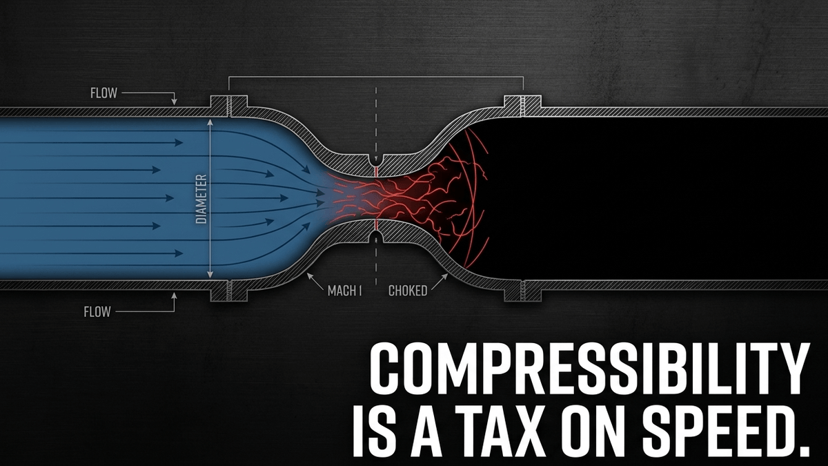
Pneumatic systems face even stricter physical boundaries. The speed of a pneumatic actuator is limited by the supply pressure and the rate at which air can move through tubes and valves. A critical limit occurs when air reaches the speed of sound at any point in the circuit. Once this "choked flow" state is reached, increasing pressure will not result in higher speeds.

Furthermore, the volume of the actuator and the friction of the piston seals create a response lag analogous to an RC (resistor-capacitor) time-delay circuit in electronics. The air must physically fill the volume and build pressure before the force overcomes static friction (stiction), creating a dead-time that software can anticipate but never eliminate.

Electrical and electromagnetic constraints

Electric actuators, while often faster than fluid-based systems, are not immune to physics. The primary constraint here is motor inertia - specifically the rotational mass of the rotor. Every time a motor changes speed, it must overcome its own internal inertia before it can deliver torque to the load. Advances in magnetic materials, such as neodymium-iron-boron magnets, allow for smaller, lighter rotors with higher flux density, but the physical mass remains a factor.

Two distinct time constants govern how an electric motor actually responds to a command, and engineers who only look at one are missing half the picture:

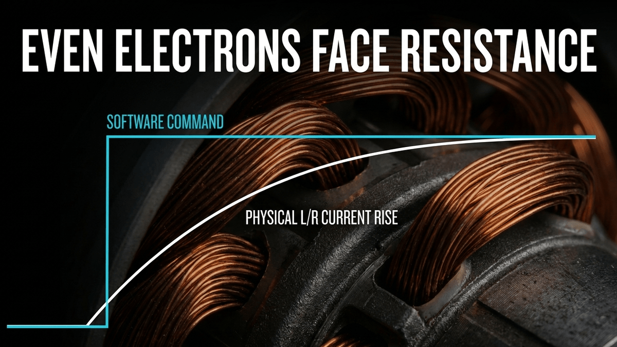
• The electrical time constant (Te) is the time needed for current in the windings to reach roughly 63.2% of its final value after a step voltage is applied, and it is set purely by the inductance and resistance of the windings.
• The mechanical time constant (Tm) is the time needed for the rotor to spin up to roughly 63.2% of its no-load speed, and it is set by the rotor's moment of inertia against available torque.

In most servo motors, the electrical time constant is the faster of the two, which is precisely why the mechanical dynamics - not the electronics - end up dominating the overall response. A well-documented example: a servo motor with a moment of inertia of 0.0179 kg·m² and 10.51 Nm of rated torque takes roughly 0.112 seconds to spin up to 63% of a 1000 rpm rated speed under its own inertia alone, before any load is even attached. Bolt that motor to a robot arm, gearbox, and end effector, and the effective mechanical time constant only grows.

This is not a theoretical concern. Field measurements on the NAO humanoid robot found a consistent motor response delay of around 30 milliseconds between a position command being issued and the motor visibly reacting, a figure that researchers traced to the combination of a 100 Hz control loop and the multi-stage communication chain between the main controller and the motor-level microcontrollers. Some joints on worn or heavily used robots showed delays closer to 40 milliseconds, hinting that mechanical wear compounds the electrical lag over a machine's service life. That is a useful reminder that latency figures on a datasheet describe a new, pristine actuator - not necessarily the one on your production floor two years from now.

Beyond mass, electrical time constants play a significant role in other actuator families too. In electrostatic actuators, the capacitive nature of the components creates a delay in charging and discharging. These dynamics are governed by the electrical RC circuit, which often limits frequency response to below a few kilohertz. Even the power electronics feeding the motor introduce latency. While modern silicon carbide (SiC) and gallium nitride (GaN) semiconductors allow for faster switching frequencies and reduced losses, the time required for current to rise in an inductive motor winding (the L/R time constant) remains a fundamental bottleneck.

Material properties and mechanical design limits

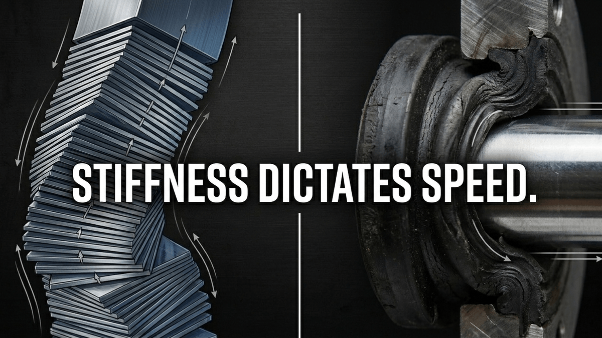
The stiffness of an actuator's materials directly impacts how quickly force is transmitted. If a material is too elastic, the actuator will "wind up" like a spring before the load moves, leading to oscillations and delayed response. For example, piezoelectric ceramics are prized for their speed, yet their modulus of elasticity is only about 25% that of steel.

This elasticity means that at extreme frequencies, the material itself can undergo delamination or structural failure if pushed beyond its mechanical strength. Furthermore, the speed of a nanopositioner is strictly limited by its first eigenfrequency (resonance). A piezo actuator can generally only reach its nominal displacement in approximately one-third of the period of its resonant frequency. If you attempt to drive the system faster, the resulting resonance will cause the system to lose precision or destroy itself.

Friction also acts as a relentless tax on speed. In linear actuators, seals required for high ingress protection (IP ratings) press against the moving rod. While this protects the internals from dust and water, it introduces significant drag. High-IP actuators are almost always slower than their unsealed counterparts because the motor must spend a portion of its torque just overcoming the friction of the rubber seals.

What biology already figured out

It is worth a brief detour into biomechanics here, because animals face the exact same latency problem and their solution is instructive. Nerve conduction delay in a cat-sized animal runs to 30 milliseconds or higher, which sounds catastrophic until you realize a full stance phase during running at 4 Hz with a 0.4 duty factor lasts only about 100 milliseconds. In other words, animals are running with a neuromuscular delay that eats nearly a third of their available reaction window, and they are not falling over.

The trick is not faster nerves. It is mechanical compliance built into the tendons and muscle-tendon units themselves, which absorb the impact of touch-down passively, before any nervous-system feedback loop even has time to respond. Modern legged robots borrow this idea directly through parallel elastic actuation, where a spring element sits alongside the motor and handles the first, fastest part of an impact so the control loop does not have to. It is the mechanical equivalent of adding a shock absorber instead of writing a faster reflex.

This matters for the "code cannot fix physics" argument because it shows the correct fix has never been a purely computational one, in biology or in engineering. The fix is structural. Add compliance where speed cannot be bought, and let the control loop handle only what it can actually keep up with.

The spectrum of actuator latency

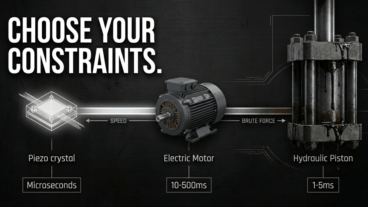
Choosing the right actuator technology is essentially a process of selecting which physical constraints you are willing to accept.

• Piezoelectric actuators: These represent the gold standard for speed. They can achieve nominal displacement in microseconds and sustain accelerations exceeding 10,000g. Their primary limit is the amplifier's slew rate and the current capacity required to charge the ceramic stack.
• Hydraulic actuators: Excellent for high-force applications, they offer response times in the 1-5 millisecond range when equipped with high-end servo valves.
• Electric actuators: These are the most common in automation, with response times typically between 10 and 500 milliseconds. Linear motors are the fastest among them, lacking the mechanical transmission (like screws or belts) that adds friction and heat, though they are usually capped at 5 m/s by the limits of their guide mechanisms.
• Pneumatic actuators: These are capable of rapid acceleration but are limited by the compressible nature of air and internal flow restrictions, generally operating effectively at speeds around 500 mm/s.

For readers weighing these trade-offs against cost, force output, and infrastructure requirements rather than latency alone, the comparison of hydraulic, electric, and pneumatic actuator types covers that ground in more depth.

Why code cannot fix physics

A common misconception in modern engineering is that a sufficiently advanced control algorithm can compensate for any hardware deficiency. This is false. While software can optimize performance within the physical limits - by reducing overshoot or using feed-forward terms to anticipate delays - it cannot change the laws of physics.

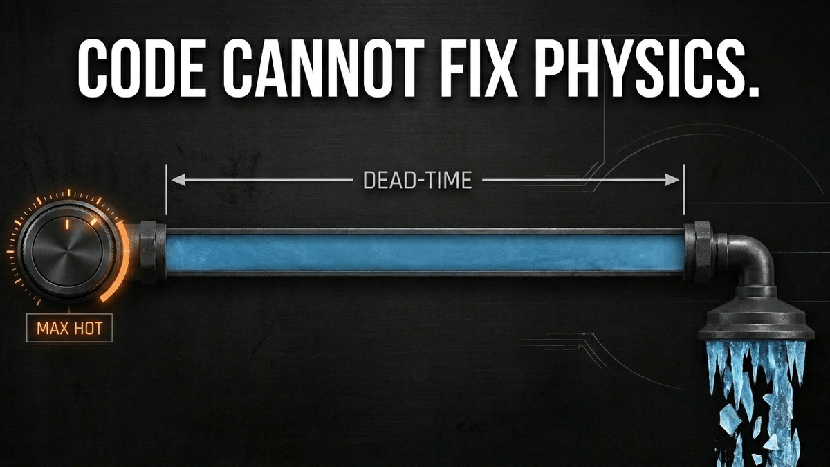
Consider the "showering person" analogy. If there is a ten-second delay between turning the knob and the water temperature changing at the showerhead, the person (the controller) will likely oscillate between freezing and scalding water. Turning the knob faster (a more aggressive software command) does not change the fact that the cold water already in the pipes (the mechanical latency) must be purged before the hot water arrives.

In robotics, total system latency is the sum of sensor delays, communication lag, processing time, and finally, actuator response. Field data from legged robot platforms shows why the ordering of this stack matters so much: proprioceptive actuators need communication and control delays in the range of a few milliseconds to support control frequencies above 500 Hz, while a camera running at 30 Hz with 50 milliseconds of latency is perfectly adequate for high-level decisions but useless for balance control. That is why a falling humanoid cannot simply "look" its way back to stability. By the time a frame is captured, transmitted, and run through a vision model, gravity has already won.

This is also why engineers deliberately design layered control architectures, with the fastest sensors - joint encoders, IMUs, force/torque sensors - feeding the innermost, highest-frequency loops, and slower sensors like cameras feeding only the outer planning loop. It is not a limitation of current AI models that they cannot run balance control directly off vision. It is a hard consequence of the physical stack: sensor readout, transit, and display or actuation all cost real time that no amount of clever software can refund.

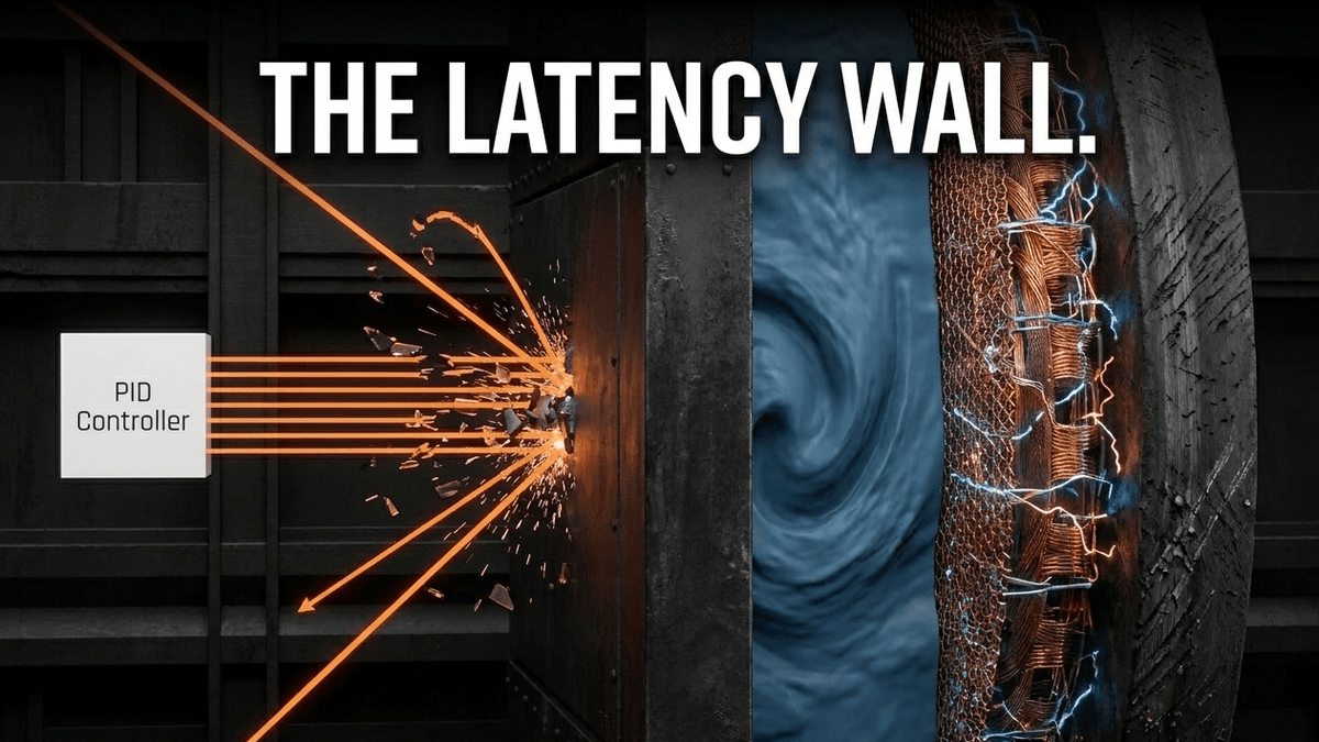
While we can reduce processing time by using real-time operating systems (RTOS) and faster protocols, the physical time required for a motor to accelerate a heavy arm remains a hard limit. If a toolpath requires a sharp corner that exceeds the jerk limits of the motor, the software must slow down. If the software forces the move, the hardware will either deviate from the path or suffer long-term mechanical fatigue.

Diagnosing latency: a practical framework

When a motion system underperforms, the diagnostic path should always separate tuning problems from physical ones before a single line of code is touched. A short, disciplined sequence works better than guesswork:

1. Measure the actual actuator response, not the datasheet figure. Wear, contamination, and temperature all degrade real-world performance below the nominal spec.
2. Decompose the loop into sensor delay, communication lag, processing time, and actuator response, and identify which single stage dominates the total. In most industrial systems, the actuator stage sets the floor - shaving microseconds off a fieldbus protocol will not matter if the valve itself needs tens of milliseconds to move.
3. Check whether the requested motion profile is physically achievable given the actuator's rated force, acceleration, and bandwidth. A jerk-limited toolpath that demands more than the hardware can deliver is not a tuning failure.
4. Only then tune the controller - adjusting PID gains, adding feed-forward terms, or refining the RTOS scheduling - to extract the best performance the hardware is physically capable of.

Skipping straight to step four is the most common mistake in the field, and it is why so many "software problems" turn out, weeks later, to be undersized motors or oversized loads.

The engineering takeaway

Industrial motion systems fail for two primary reasons: either the controls are poorly tuned, or the mechanics are physically incapable of producing the requested profile. The first issue is a software problem and can be fixed in the field with a laptop and an experienced engineer. The second issue is a fundamental design failure. If the mass is too high, the motor too small, or the fluid too compressible for the required cycle time, no amount of code will solve the problem.

Success in motion control requires a detached, data-driven approach to hardware selection. One must respect the F=ma equation and the thermal limits of the materials. When the physics of the actuator cannot meet the demands of the application, the only solution is to change the physics - by reducing mass, increasing stiffness, or switching to a more responsive actuator technology. Code is a powerful tool for orchestration, but physics is the ultimate conductor.

That gap between what code executes and what mass can physically do is not a bug to be patched. It is the design boundary every motion engineer works within, whether they are speccing a piezo stack for a wafer stepper or a hydraulic ram for a forging press.